why linear algebra?

linear algebra is the study of linear maps: functions that preserve addition and scaling.

• if you double the input → the output doubles
• if you add two inputs → the outputs add

in math terms, for a linear map ( f ):

\[\color{#2062b8}{f(c \mathbf{v}) = c f(\mathbf{v}) \quad \text{for any number } c}\] \[\color{#2062b8}{f(\mathbf{v}_1 + \mathbf{v}_2) = f(\mathbf{v}_1) + f(\mathbf{v}_2)}\]

these rules might sound abstract, but they actually describe real operations that show up everywhere: stretching, rotating, shearing or flipping space. you’ll find them in physics (forces), graphics (rotations, scaling) and in a neural network.

---

seeing linear maps in action: transformation matrices

in two dimensions, a 2×2 matrix is the most direct way to describe a linear map.

the interactive demo below lets you see this in action:

• use the sliders to change how each point on the grid moves
• each slider controls one entry in a 2×2 matrix
• as you adjust the matrix, you create a new linear map

what do the sliders do?
- a₁₁: controls stretching/compression or flipping along the x direction.
- a₁₂: mixes the y value into the new x (shearing/rotation).
- a₂₁: mixes the x value into the new y (shearing/rotation).
- a₂₂: controls stretching/compression or flipping along the y direction.

these four sliders make a 2×2 matrix:
[ a₁₁  a₁₂ ]
[ a₂₁  a₂₂ ]

this matrix transforms every point (x, y) to (a₁₁x + a₁₂y, a₂₁x + a₂₂y).
experiment with the sliders to see stretches, shears, rotations, and reflections! the multiplication \(A \mathbf{x}\) works like this: \[ A = \begin{bmatrix} a_{11} & a_{12} \\ a_{21} & a_{22} \end{bmatrix} , \quad \mathbf{x} = \begin{bmatrix} x \\ y \end{bmatrix} \] multiplying \(A\) by \(\mathbf{x}\) means taking the dot product of each row of \(A\) with \(\mathbf{x}\): \[ A \mathbf{x} = \begin{bmatrix} a_{11} & a_{12} \\ a_{21} & a_{22} \end{bmatrix} \begin{bmatrix} x \\ y \end{bmatrix} = \begin{bmatrix} a_{11} \cdot x + a_{12} \cdot y \\ a_{21} \cdot x + a_{22} \cdot y \end{bmatrix} \] a dot product is an operation that takes two equal-length vectors and returns a single number by multiplying corresponding entries together and then summing those products. in the case of matrix multiplication, you take the dot product of each row of the matrix with the input vector. since the matrix has two rows, you get two dot products, one per row, resulting in a new vector with two components. each component shows how much the input vector projects onto that row’s direction, giving the transformed coordinates.

the effect you see on the grid is exactly what happens when your transformation matrix ie. a linear map is applied to every vector on the plane. the power of linear maps: no matter how the grid morphs, straight lines remain straight and the origin never moves.

---

kernel, rank and degrees of freedom

Every linear map \(\color{#2062b8}{ f : \mathbb{R}^n \to \mathbb{R}^m }\) where n is the number of input variables (dimensions in the domain) and m is the number of output variables (dimensions in the codomain), can be represented by a matrix

\(\color{#2062b8}{ A \in \mathbb{R}^{m \times n} .}\) The kernel (null space) of ( f ) is the set of all input vectors sent to zero when the linear map is applied:

This kernel consists of all solutions to the homogeneous system:

The rank of ( f ) is the dimension of its image (the set of outputs you can reach by applying ( f )):

The dimension of the kernel tells us how many degrees of freedom remain after applying the constraints, so they are like free variables which can vary independently and are defined by ( f ):

If all constraints are independent ( \(\operatorname{rank}(f) = m\)), then

rank-nullity theorem

the rank-nullity theorem links kernel and rank for any linear map: \(\operatorname{rank}(f) + \operatorname{nullity}(f) = n\) where \(\operatorname{nullity}(f) = \dim(\ker(f))\)

so, the number of independent constraints (rank) plus the number of free directions (nullity) always equals the number of variables. if rank goes up, nullity goes down—your degrees of freedom are reduced. this is why counting kernel and rank gives you the full picture of which directions survive after constraints.

geometric intuition:

• ( n ): number of variables = initial degrees of freedom
• ( m ): number of independent equations = constraints reducing freedom

the interactive demo shows how a 2×2 matrix acts as a linear map. when you use a matrix for a linear map, each constraint cuts down your degrees of freedom. the kernel is the set of directions(yes think vectors) that get collapsed to zero by those constraints. the rank tells you how many constraints are actually independent.

as you add more constraints, you lose freedom. fewer constraints means more freedom. your degrees of freedom are the directions left after the linear map acts.

isomorphisms: when nothing gets lost

after seeing how constraints reduce degrees of freedom, we naturally ask: what happens when we can fully reverse a transformation? this brings us to isomorphisms—the “perfect translators” of linear algebra.

an invertible linear map (isomorphism) is like having a perfect translator between two vector spaces, nothing gets lost in translation, and you can always go back to the original. in our degrees of freedom language: an isomorphism preserves all degrees of freedom.

the three conditions that lock together

in finite dimensional spaces, these three properties are completely equivalent and they are exactly what you need for isomorphisms.:

\[\color{#2062b8}{\text{injective} \iff \text{surjective} \iff \text{invertible}}\]

• injective (one-to-one): different inputs give different outputs
• surjective (onto): every possible output is reached ie. range is equal to the codomain (think about it :p)
• invertible: you can undo the transformation

remember our formula \(\dim(\ker(f)) = n - \operatorname{rank}(f)\) ? for isomorphisms between spaces of the same dimension, we need the kernel to be trivial (only the zero vector) and the rank to be maximal. this forces both injectivity and surjectivity.

bases: your lens for viewing spaces

here’s where things get strategic. every vector space has infinitely many possible bases - minimal sets of independent vectors that can build everything else through scaling and addition.

think of a basis as your “lens” for viewing a vector space. once you know how a linear map transforms each basis vector, you know how it transforms every vector in the space.

wait, we have’nt yet discussed what a vector space is atleast formally right

a vector space is like a playground for vectors — objects you can add together and stretch or shrink by numbers (scalars). the main idea is: no matter how you combine or scale them, you’re always still playing in the same space. think of it as a set of arrows, or lists of numbers, or even functions, where you can mix and scale things any way you like, and you never have to leave the playground. this simple set of rules is the foundation for all of linear algebra!

the three mindsets for choosing your lens

1. fixed lens (limiting): stick to standard coordinates (x, y, z axes). useful for computation but hides structure.

2. no lens (abstract): work purely with abstract maps and concepts. mathematically pure but hard to visualize for normal folks like me ;-;.

3. strategic lens (optimal): choose your basis to fit the problem structure. this is what you want to master.

the strategic approach means reading your problem carefully, identifying the important subspaces or transformations, then choosing a basis that makes those structures obvious.

building better bases: steinitz exchange theorem

if you have a linearly independent set u with k vectors and a spanning set w for the vector space, you can replace exactly k vectors from w with the vectors from u and the new set will still span the space. the independent set u doesn’t need to be a basis, and the replacements always come from the spanning set w.

this means any independent set can be extended to a basis by adding vectors from a spanning set, which is a fundamental tool for understanding and building bases.

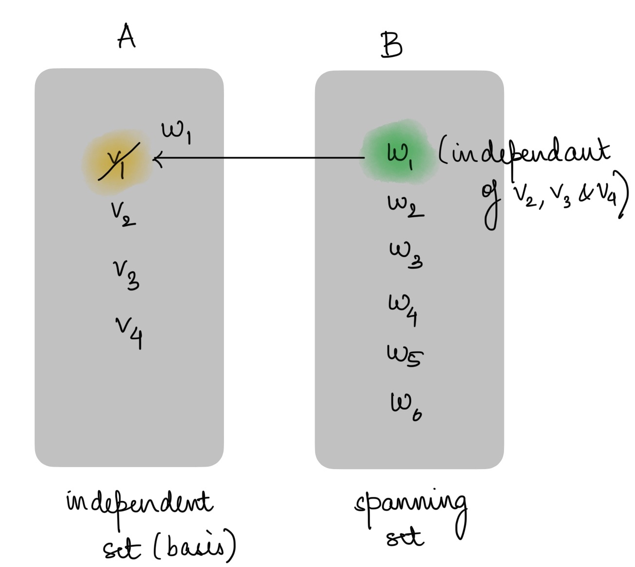
The new set in this image after adding w₁ is still a basis for that vector space

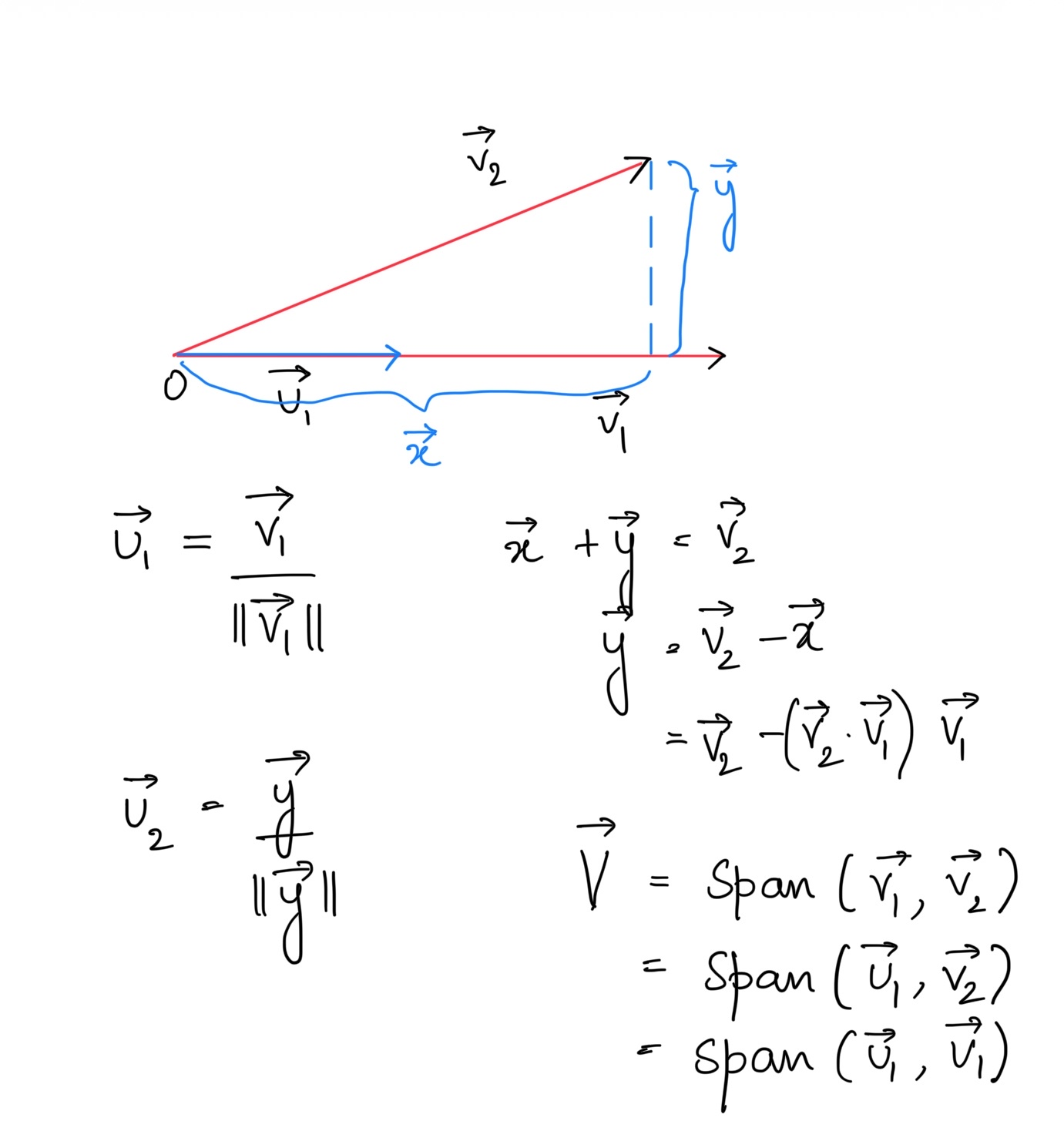
gram-schmidt process

the gram-schmidt process transforms any basis into an orthonormal basis—vectors that are mutually perpendicular and have unit length. this is crucial for numerical stability in machine learning algorithms.

For a 2d vector space:

After these steps,

is an orthonormal basis spanning the same space as \(\{\vec{v}_1,\vec{v}_2\}\).

---

with love